
This is the 14th article in our series on data quality problems for process mining. You can find an overview of all articles in the series here.
Disco detects parallelism if two activities for the same case overlap in time. Usually, this is exactly what you want. If you have a process that contains parallel activities, these activities cannot be displayed in sequence because this is just not what happens.
However, sometimes activities can overlap in time due to data quality problems. For example, if you look at the ‘Case 1’ below then you see that activities B and C overlap by just 1 second. The process mining tool sees that both activities are (partially) going on at the same time and shows them in parallel.
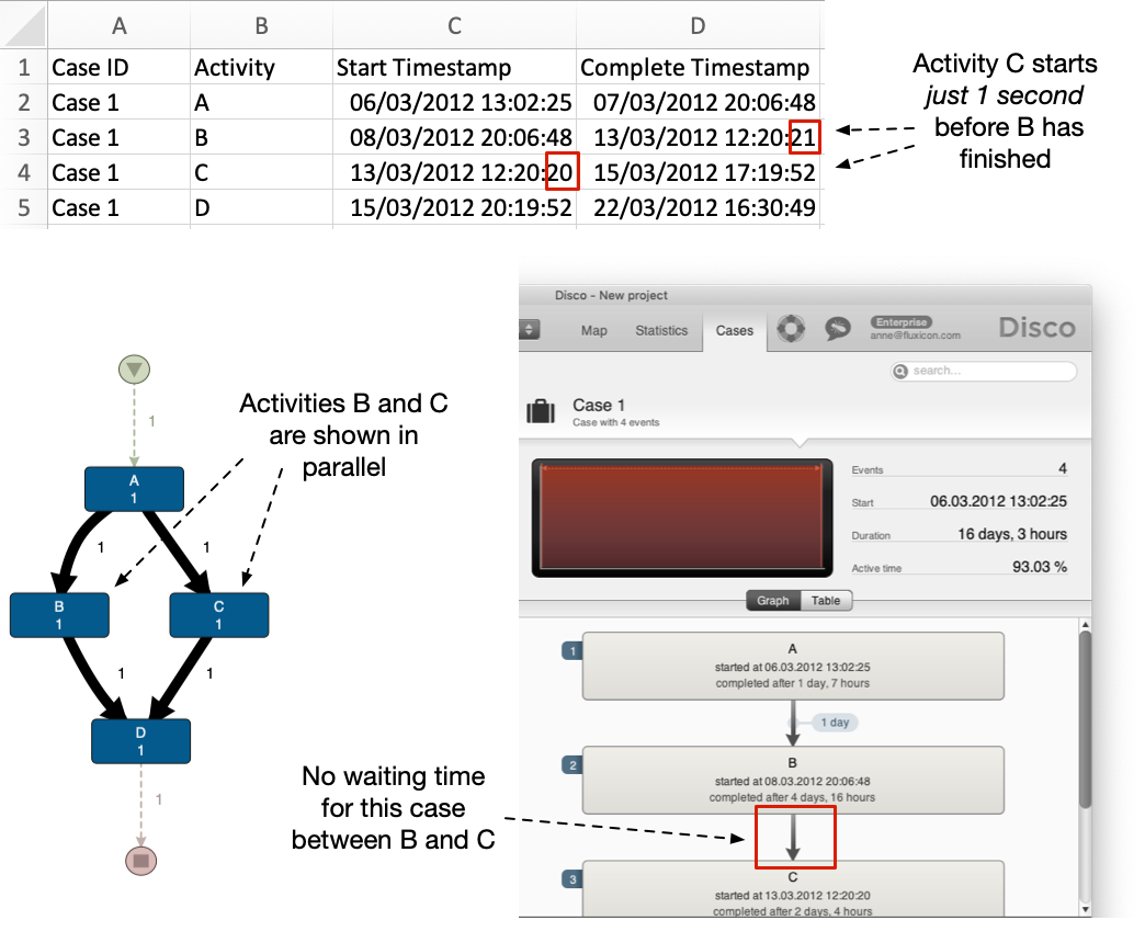
If you expect your process to be sequential, parallelism may be due to the way that the data is recorded. For example, for ‘Case 1’ above the Complete Timestamp for activity B might have been supposed to be the same as the Start Timestamp for activity C, but they were written by the logging mechanism one after the other, or the writing of the Complete Timestamp for activity B might have been delayed by the network in a distributed system.
So, if the process that you have discovered is different from what you expected it to be, it is worth investigating whether you are dealing with parallel activities.
One way to see that you are dealing with parallelism is that the frequency numbers in the process map add up to more than 100%. For example, in the process map above activity A has the frequency 1 but the frequencies at the outgoing arcs add up to 2 (because both parallel branches are entered in parallel). Another way to see this is by switching to the Graph view in the Cases tab, which will not show you any waiting time between activities that overlap in time (if there is 0 time between them the waiting time will be shown as ‘instant’).
How to fix:
First, investigate individual parallel cases to understand the extent and the nature of the parallelism in your process (see below). For example, it could be that parts of your process are actually happening in parallel while you expected the process to be sequential.
If you are sure that the parallelism is due to a data quality problem, you can create a sequential view of your process by choosing just one timestamp column during the import step (see below).
To fully resolve unintended overlapping timestamps for activities that should be recorded in sequence, you need to go back to the data source and correct the timestamps before you import the data again into Disco with both timestamps. Ultimately, the logging mechanism needs to be fixed to prevent the problem to re-occur in the future.
Both of the following strategies can also be useful to better understand processes that actually have legitimate parallel parts in them. Parallel processes are often much more complicated to understand and it can help to look at example cases and at sequential views to better understand the (correct but still complicated) parallel process views.
1. Explore individual parallel cases
When you look at an individual case in the process map for a sequential process, the result is quite boring because you will see just a sequence of activities (unless there is a loop in the process). However, in parallel processes each case can have activities that are performed independently of each other. So, the process map for even a single case can become quite complex.
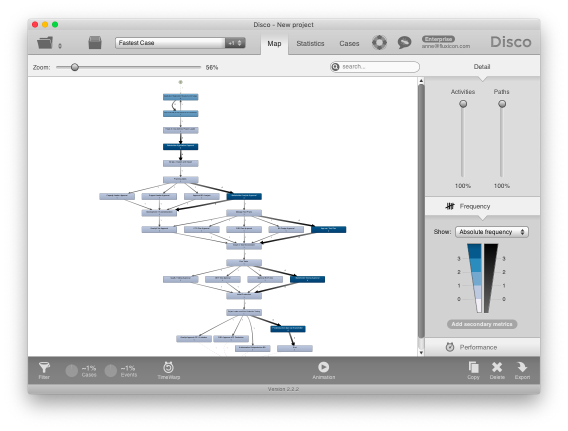
To fully understand this, it helps to look at an individual case in isolation. For example, in a project management process that contains a lot of parallel activities we might choose to look at the fastest case to get an idea of what the process flow has looked like in the best case. To do this, we sort the cases based on the duration and use the short-cut ‘Filter for case …’ via right-click to automatically add a pre-configured Attribute filter for this case. We can then save this view with the name ‘Fastest case’ (see screenshot below - click on the image to see a larger version of it).

After applying the filter, we can see the process map for just this one case. Although we are looking at a single case, the process map does not just show a sequential flow but a process with parallel activities in several phases (see below).
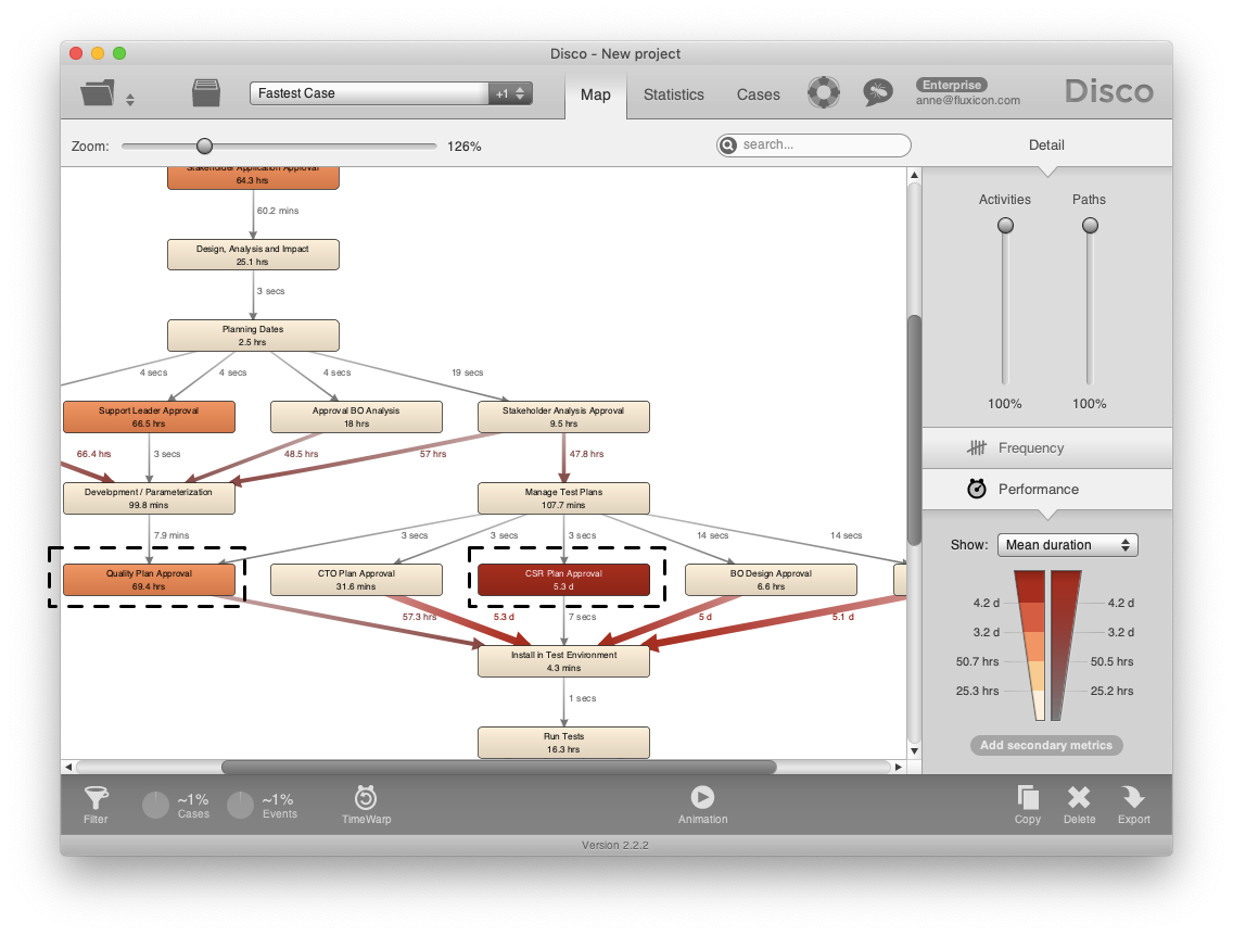
When we look at the performance view, we can see that out of the 5 activities that are performed in parallel between the ‘Manage Test plans’ and the ‘Install in Test Environment’ milestones the ‘Quality Plan Approval’ and the ‘CSR Plan Approval’ steps take the longest time (see below).
When we animate this single case, we see the parallel flows represented by individual tokens as well. For example, in the screenshot below, we can see that on Sunday 20 May the ‘Quality Plan Approval’ and the ‘CSR Plan Approval’ activities were still ongoing (see blue token in activity) while the other three activities had already been finished (see yellow tokens between activities).

In contrast, when we look at the slowest case in this project management process then we observe that the most time is spent in a later part of the process, namely the ‘Run Tests’ activity (see below).

Tip: To view multiple parallel cases - still isolated from each other - next to each other, you can duplicate the case ID column in the source data and import your data again with the duplicated column configured as part of the activity name. You will then see the process maps for all the individual cases next to each other. Of course, this will be too big for all cases, but you can then again focus on a subset by filtering, e.g, 2 or 3 cases and look at them together.
This will provide you a relative comparison for the performance views. Furthermore, you can use the synchronized animation to compare the dynamic flow across the selected cases with a relative start time in the animation.
2. Import sequential view of the process
To completely “turn off” the parallelism in the process map, you can simply import your data set again and configure only one of your timestamps as a ‘Timestamp’ column. If you have only one timestamp configured, Disco always shows you a sequential view of your process. Even if two activities have the same timestamp they are shown in sequence with ‘instant’ time between them.
Looking at a sequential view of your process can be a great way to investigate the process map and the process variants without being distracted by parallel process parts. Furthermore, taking a sequential view can be a quick fix for a data set that has unwanted parallelism due to a data quality problem as shown above.
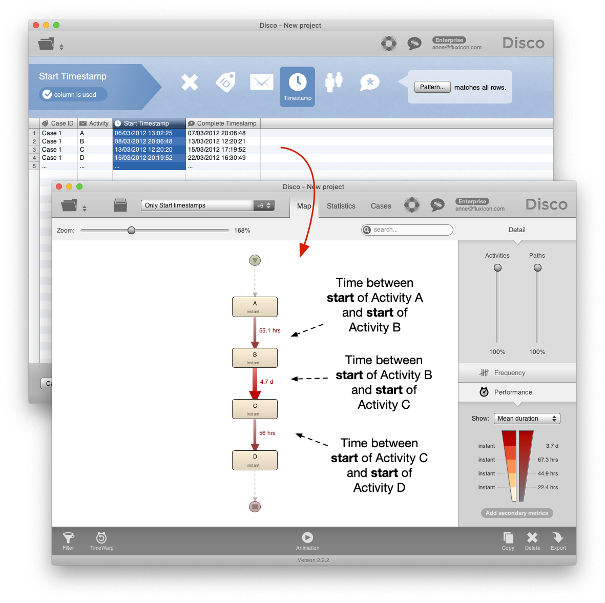
If we want to take a sequential view on the example Case 1 from the beginning of this article, we can choose either the ‘Start Timestamp’ or the ‘Complete Timestamp’ as a timestamp during the import step. Keep in mind that the meaning of the waiting times in the process map changes depending on which of the timestamps you choose.
For example, if only the ‘Start Timestamp’ column is configured as ‘Timestamp’ during the import step, then the resulting process map shows a sequential view of the process for Case 1. Because there is only one timestamp per activity, the activities themselves have no duration (shown as ‘instant’). The waiting times reflect the times between the start of the previous activity until the start of the following activity (see below).
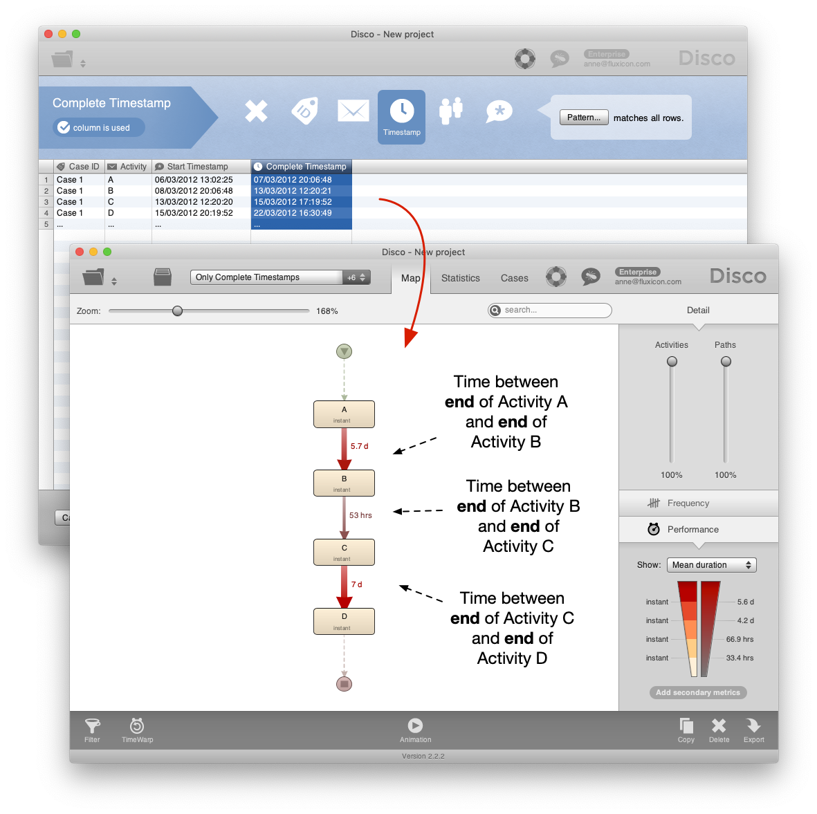
In contrast, when the ‘Complete Timestamp’ column is chosen as the timestamp then the waiting times will be shown as the durations between the completion times of the activities (see below).
So, keep this in mind when you interpret the performance information in your sequential process map after importing the data again with a single timestamp. 1
To sum it up, parallel processes can cause headaches due to their increased complexity quite quickly. Try the two strategies above and don’t forget to also apply the regular simplification strategies to explore what helps best to give you the most understandable view. For example, looking at different process phases of the process in isolation and taking a step back by focusing on the milestone activities can be really useful. All these strategies can also be combined with each other.
-
Note that the order of the events in a case - and, therefore, the variants - might change when you change the import perspective from ‘start’ timestamp to ’end’ timestamp (or the other way around) as well. ↩︎

Anne Rozinat
Market, customers, and everything else
Anne knows how to mine a process like no other. She has conducted a large number of process mining projects with companies such as Philips Healthcare, Océ, ASML, Philips Consumer Lifestyle, and many others.